Electrical conductivity of graphite
In this project the electronic dispersion $E(\vec{k})$ of graphite are derived from a density functional theory (DFT) calculation using VASP and from a tight binding model. From the discreet $E(\vec{k})$ dispersion relation the two non zero elements of the conductivity tensor of graphite are calculated by a numerical integration of the corresponding Boltzmann equation.
The DFT calculation
In the DFT calculation the basis vectors of the hexagonal unit cell are chosen as
\begin{equation}
\vec{a}_1 = a \left[ {\begin{array}{c} 1 \\ 0 \\ 0 \end{array} } \right] ,\;
\vec{a}_2 = a \left[ {\begin{array}{c} -1/2 \\ \sqrt{3}/2 \\ 0 \end{array} } \right] ,\;
\vec{a}_3 = c \left[ {\begin{array}{c} 0 \\ 0 \\ 1 \end{array} } \right] ,
\end{equation}
and therefore the reciprocal lattice vectors are given by
\begin{equation}
\vec{b}_1 = \frac{2 \pi}{a} \left[ {\begin{array}{c} 1 \\ 1/\sqrt{3} \\ 0 \end{array} } \right] ,\;
\vec{b}_2 = \frac{2 \pi}{a} \left[ {\begin{array}{c} 0 \\ 2/\sqrt{3} \\ 0 \end{array} } \right] ,\;
\vec{b}_3 = \frac{2 \pi}{c} \left[ {\begin{array}{c} 0 \\ 0 \\ 1 \end{array} } \right] ,
\end{equation}
which again give a hexagonal lattice. The four carbon atoms in the unit cell are positioned at
\begin{equation}
p_1 = \left[ {\begin{array}{c} 0 \\ 0 \\ 1/4 \end{array} } \right] ,\;
p_2 = \left[ {\begin{array}{c} 1/3 \\ 2/3 \\ 1/4 \end{array} } \right] ,\;
p_3 = \left[ {\begin{array}{c} 0 \\ 0 \\ 3/4 \end{array} } \right] ,\;
p_4 = \left[ {\begin{array}{c} 2/3 \\ 1/3 \\ 3/4 \end{array} } \right] ,
\end{equation}
with respect to the base vectors. In the calculation for every carbon atom 4 valence electrons are included, which means 16 electrons per unit cell. By searching a minimum in total energy the lattice parameter are determined as $a = 2.46598 \; A$ and $a = 6.44 \; A$. Using this lattice parameter the $E(\vec{k})$ relation in the first Brillouin zone is determined on a equidistant 41x41x12 grid along the basis vectors, with 12 energy values for each $\vec{k}$-point. Hence 12 bands are calculated with 8 of them occupied, the band structure along some high symmetry lines is plotted in the following figure.
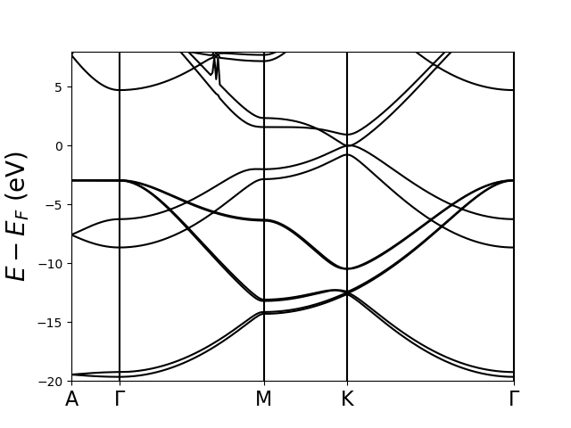
This plot shows band structure of graphite along some high symmetry lines using a DFT calcualtion.
In the following figure the resulting density of states (DOS) are plotted.
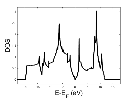
This plot shows the density of states of graphite as given in the DOSCAR file of the DFT calculation using VASP.
The Fermi energy is at $E_F = 5.04 \; eV$. Since the DOS are nearly symmetric around the Fermi energy, the chemical potential is almost constant with temperature and for further calculations the chemical potential is approximated by the Fermi energy. The calculated $E(\vec{k})$ dispersion relation from the EIGENVAL file is read in by the following Matlab function.
The tight binding model
The tight binding model as described by Wallace was used as a second approach to get the $E(\vec{k})$ dispersion relation. In this model just the $p_z$ electron is included in the calculation, with leads to 4 electrons per unit cell. Additionally I ignore all parameters except $\gamma_0$ and $\gamma_1$, which gives the four bands
\begin{equation}
E(\vec{k}) = \pm \frac{1}{2} \gamma_1 \Gamma(\vec{k}) \pm \sqrt{\frac{1}{4} \gamma_1^2 (\Gamma(\vec{k}))^2 + \gamma_0^2 \left|S(\vec{k})\right|^2} ,
\end{equation}
with
\begin{equation}
\Gamma(\vec{k}) = 2 \cos\left(\frac{c}{2} k_z\right),
\end{equation}
\begin{equation}
\left|S(\vec{k})\right|^2 = 1 + 4 \cos^2\left(\frac{a}{2} k_x\right) + 4 \cos\left(\frac{a}{2} k_x\right) \cos\left(\frac{\sqrt{3} a}{2} k_y\right).
\end{equation}
The remaining two tight binding parameter are taken from Tung , with $\gamma_0 = 3.18 \; eV$ and $\gamma_1 = 0.38 \; eV$. The discrete $E(\vec{k})$ dispersion relation in the tight binding model and the corresponding density of states are calculated using the following Matlab function.
The resulting density of states are plotted in the following figure.
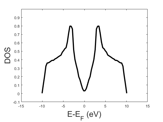
This plot shows the density of states of graphite derived from the tight binding model.
Calculation of the conductivity tensor
As graphite has a hexagonal crystal lattice the rank 2 conductivity tensor has only 3 non zero entries which are $\sigma_{11} = \sigma_{22}$ and $\sigma_{33}$. Hence it is sufficient to calculate $\sigma_{22}$ and $\sigma_{33}$. In the Boltzmann approximation the diagonal tensor elements are given as
\begin{equation}
\sigma_{jj} = \frac{e^2}{\pi h^2} \int \tau(\vec{k},T) \frac{\partial f_0}{\partial \mu} \left(\vec{\nabla}_{\vec{k}} E(\vec{k}) \cdot \vec{e}_j \right)^2 d^3k \;,
\end{equation}
with
\begin{equation}
\frac{\partial f_0}{\partial \mu} = \frac{1}{k_b T} \frac{\exp{\left(\frac{E - \mu}{k_b T}\right)}}{\left(1 + \exp{\left(\frac{E - \mu}{k_b T}\right)}\right)^2} \;.
\end{equation}
For a coordinate transformation to $b_1$, $b_2$ ,$b_3$, the coordinates with respect to the reciprocal lattice vectors, the Jacobian determinant is given by
\begin{equation}
\left|J\right| = \frac{16 \pi^3}{\sqrt{3} a^2 c} \;.
\end{equation}
Furthermore the partial derivatives are given by
\begin{equation}
\frac{\partial E(\vec{k})}{\partial k_x} = \sum_j \frac{\partial E(\vec{b})}{\partial b_j} \frac{\partial b_j}{\partial k_x} = \frac{a}{2 \pi} \frac{\partial E(\vec{b})}{\partial b_1} - \frac{a}{4 \pi} \frac{\partial E(\vec{b})}{\partial b_2} \;,
\end{equation}
\begin{equation}
\frac{\partial E(\vec{k})}{\partial k_y} = \sum_j \frac{\partial E(\vec{b})}{\partial b_j} \frac{\partial b_j}{\partial k_y} = \frac{\sqrt{3} a}{4 \pi} \frac{\partial E(\vec{b})}{\partial b_2} \;,
\end{equation}
\begin{equation}
\frac{\partial E(\vec{k})}{\partial k_z} = \sum_j \frac{\partial E(\vec{b})}{\partial b_j} \frac{\partial b_j}{\partial k_z} = \frac{c}{2 \pi} \frac{\partial E(\vec{b})}{\partial b_3} \;.
\end{equation}
Consequently the two tensor elements are given by
\begin{equation}
\sigma_{22} = \frac{e^2}{\pi h^2} \int \tau(\vec{b},T) \frac{\partial f_0}{\partial \mu} \frac{3 a^2}{16 \pi^2} \left(\frac{\partial}{\partial b_2}E(\vec{b})\right)^2 \frac{16 \pi^3}{\sqrt{3} a^2 c} d^3b \;,
\end{equation}
\begin{equation}
\sigma_{33} = \frac{e^2}{\pi h^2} \int \tau(\vec{b},T) \frac{\partial f_0}{\partial \mu} \frac{c^2}{4 \pi^2} \left(\frac{\partial}{\partial b_3}E(\vec{b})\right)^2 \frac{16 \pi^3}{\sqrt{3} a^2 c} d^3b \;.
\end{equation}
Now it remains to find a approximation for the relaxation time $ \tau(\vec{k},T) $, respectively the free path length $ l(T) $ with $ \tau(\vec{k},T) = v(\vec{k}) l(T)$. In literature usually the relaxation time is split up into two parts
\begin{equation}
\frac{1}{\tau(\vec{k},T)} = \frac{1}{\tau_{def}(\vec{k})} + \frac{1}{\tau_{ph}(\vec{k},T)} = \frac{v(\vec{k})}{l_{def}} + \frac{v(\vec{k})}{l_{ph}(T)}
\end{equation}
with a temperature independent part $\tau_{def}(\vec{k})$ due to defects and a temperature dependant part $\tau_{ph}(\vec{k},T)$ due to interactions with photons. For graphite Kinchin found that $l_{def}$ is about 1000 A and he gave some tabulated values for $l_{ph}(T)$ in a broad temperature range from 4.2 K to 1273 K. As the function $l_{ph}(T)$ has to diverge at 0 K and the values for height temperatures seem to decay exponentially I assume a behavior like
\begin{equation}
l_{ph}(T) = \left(p_0 + \frac{p_1}{T} + \frac{p_2}{T^2} + \frac{p_3}{T^3} \right) \exp(p_4 T) \;,
\end{equation}
which is fitted to the tabulated values by the following Matlab function.
The resulting fit parameters are $p_0 = 3.27e+3 \; A$, $p_1 = 5.34e+5 \; AK$, $p_2 = 9.65e+6 \; AK^2$, $p_3 = 3.24e+8 \; AK^3$, $p_4 = -2.94e-3 \; 1/K$. In the following figure the tabulated values are plotted together with the assumed function.
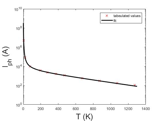
This plot shows the tabulated values of the phonon contribution of the free path length and the fitted function.
As the assumed function describes the tabulated values quite well, this function is used interpolate between the tabulated values. Now the tensor elements can be calculated by using the chosen discretization of $b_1$ = (-20,...,20)/41, $b_2$ = (-20,...,20)/41, $b_3$ = (-5,...,6)/12 from the DFT calculation for the numerical integration. The tensor elements are then given by
\begin{equation}
\sigma_{22} = \frac{e^2}{\pi h^2} \frac{\sqrt{3} \pi}{c} \frac{1}{41 \cdot 41 \cdot 12} \sum_{bands,j} \sum_{b_1} \sum_{b_2} \sum_{b_3} \left(\frac{v(\vec{k})}{l_{def}} + \frac{v(\vec{k})}{l_{ph}(T)}\right)^{-1} \frac{\partial f_0}{\partial \mu} \left( \frac{\partial}{\partial b_2}E_j(\vec{b})\right)^2 \;,
\end{equation}
\begin{equation}
\sigma_{33} = \frac{e^2}{\pi h^2} \frac{4 \pi c}{\sqrt{3} a^2} \frac{1}{41 \cdot 41 \cdot 12} \sum_{bands,j} \sum_{b_1} \sum_{b_2} \sum_{b_3} \left(\frac{v(\vec{k})}{l_{def}} + \frac{v(\vec{k})}{l_{ph}(T)}\right)^{-1} \frac{\partial f_0}{\partial \mu} \left(\frac{\partial}{\partial b_2}E_j(\vec{b})\right)^2 \;,
\end{equation}
with the velocity $v(\vec{k})$ approximated by
\begin{equation}
v(\vec{k}) = \frac{2 \pi}{h} \left|\vec{\nabla}_{\vec{k}} E(\vec{k}) \right| = \frac{2 \pi}{h} \sqrt{ \left(\frac{\partial E(\vec{k})}{\partial k_x} \right)^2 + \left(\frac{\partial E(\vec{k})}{\partial k_y} \right)^2 + \left(\frac{\partial E(\vec{k})}{\partial k_z} \right)^2} = \frac{1}{h} \sqrt{ a^2 \left(\frac{\partial E(\vec{b})}{\partial b_1} - \frac{1}{2} \frac{\partial E(\vec{b})}{\partial b_2}\right)^2 + \frac{3 a^2}{4} \left(\frac{\partial E(\vec{b})}{\partial b_2} \right)^2 + c^2 \left(\frac{\partial E(\vec{b})}{\partial b_3} \right)^2}\;,
\end{equation}
and the partial derivatives approximated by
\begin{equation}
\frac{\partial}{\partial b_1}E_j(b_1(i),b_2(j),b_3(m)) = \frac{E_j(b_1(i+1),b_2(j),b_3(m)) - E_j(b_1(i-1),b_2(j),b_3(m))}{2 \cdot 41} \;,
\end{equation}
\begin{equation}
\frac{\partial}{\partial b_2}E_j(b_1(i),b_2(j),b_3(m)) = \frac{E_j(b_1(i),b_2(j+1),b_3(m)) - E_j(b_1(i),b_2(j-1),b_3(m))}{2 \cdot 41} \;,
\end{equation}
\begin{equation}
\frac{\partial}{\partial b_3}E_j(b_1(i),b_2(j),b_3(m)) = \frac{E_j(b_1(i),b_2(j),b_3(m+1)) - E_j(b_1(i),b_2(j),b_3(m-1))}{2 \cdot 12} \;.
\end{equation}
The approximate gradient is calculated by the following Matlab function.
And the diagonal elemets of the conductivity tensor are calculated by the following Matlab function.
The results
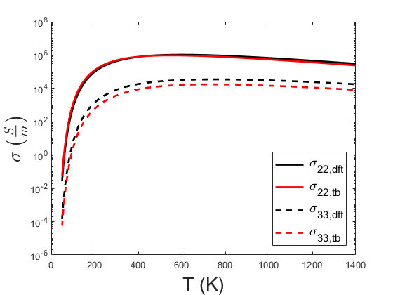
In this plot the calculated tensor elements are shown over a wide temperature range on a logarithmic scale. It can be seen that for low temperatures the conductivity goes to 0, as less and less states are contributing in the transport equation. The conductivity reaches its maximum between 500 K and 600 K and decays exponentially for higher temperature, due to the exponential law in the used approximation for the temperature dependent relaxation time. At room temperature (20°C) the calculated conductivity $\sigma_{22}$ is 4.1e+5 S/m (DFT) / 4.6e+5 S/m (tight binding), which fits in the order of magnitude to the value of 2e+5-3e+5 S/m given on Wikipedia , the calculated conductivity $\sigma_{33}$ is 7.7e+3 S/m (DFT) / 3.5e+3 S/m (tight binding), which is about a factor 10 higher than the value of 3.3e+2 S/m given on Wikipedia .
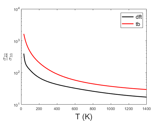
In this plot the the ratio $\sigma_{22}/\sigma_{33}$ is shown. It can be seen that the ratio increases for lower temperatures, since the in-plane conductivity $\sigma_{22}$ corresponds to the semimetal graphene, while the perpendicular conductivity $\sigma_{33}$ describes an insulator.
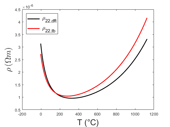
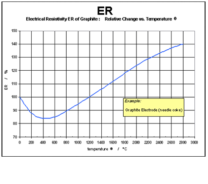
Here the calculated in-plane resistivity $\rho_{22}$ is plotted on the left hand side and compared with a graphic from the website of the European Carbon and Graphite Association on the right. When comparing the two figures, one can see that the shape of the curves is quiet similar and that the minimum is shifted by about 100 °C.