1. Magnetic susceptibility of a free-electron gas
- A free-electron gas is a system of non-interacting fermions. How could you calculate the magnetic susceptibility of a free-electron gas? Make a sketch of the magnetic susceptibility vs. magnetic field B. At high magnetic fields, the magnetization approaches a constant. Why does this happen?
Solution
A free-electron gas is a system of non-interacting fermions. How could you calculate the magnetic susceptibility of a free-electron gas? Make a sketch of the magnetic susceptibility vs. magnetic field B. At high magnetic fields, the magnetization approaches a constant. Why does this happen?
The magnetic susceptibility of free electron can be calculated with this formula:
\begin{equation*} \chi = \frac{2}{3}\mu_0 \mu_B^2 D(E_F) \end{equation*}where $D(E_F)$ is the density of states at the Fermi energy. This equation takes into account the paramagnetic (Pauli paramagnetism) and diamagnetic (Landau diamagnetism) contribution to the response of free electrons.
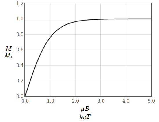
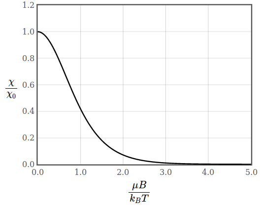 Figure 1: Magnetization and magnetic susceptibility of free electrons.
At high magnetic fields all spins are aligned with the applied magnetic field and the paramagnetic magnetization reaches saturation. Also the diamagnetic contribution saturates once all electrons are in the lowest Landau level.
2. Frequency-dependent magnetic susceptibility
To plot the frequency response of the magnetic susceptibility of a paramagnet, consider how a paramagnet would respond if an magnetic field were pulsed on and off.
- Plot the real and imaginary parts of the magnetic susceptibility of a paramagnet. Explain why the susceptibility has the form that you have drawn.
- Make a similar plot of the frequency dependence of the magnetic susceptibility of a diamagnet.
3. Ferromagnetism
- Explain how the exchange energy leads to ferromagnetism.
- What is mean field theory? How is mean field theory used to calculate the Curie-Weiss law?
- How was Landau's theory of phase transitions used to calculate the Curie-Weiss law?
Solution
Explain how the exchange energy leads to ferromagnetism.
The exchange energy is the difference in energy between the symmetric solution and the anti symmetric solution of multielectron wavefunctions. There is only a difference if the electron-electron interaction term is included.
In ferromagnets, the antisymmetric state has a lower energy. Thus the state with parallel spins has lower energy. The direct interaction between magnetic dipoles are weak compared to the exchange interaction.
In antiferromagnets, the symmetric state has a lower energy. Neighbouring spins are antiparallel.
What is mean field theory? How is mean field theory used to calculate the Curie-Weiss law?
The main idea of mean field theory (MFT) is to replace all interactions to any one body with an average or effective interaction, sometimes called a molecular field. This reduces any multi-body problem into an effective one-body problem.
Ferromagnetism can be modeled with the Heisenberg Hamiltonian
\begin{equation*} H = -\sum\limits_{i,j} J_{ij}\vec{S}_i\cdot\vec{S}_j - g\mu_B \vec{B}\cdot\sum\limits_i\vec{S}_i \ , \end{equation*}where $\vec{S}_i$ is the spin operator at lattice site $i$ and $J_{ij}$ describes the exchange energy between neighboring spins. The mean field approximation consists in replacing the interaction $\vec{S}_i\cdot\vec{S}_j$ by the interaction of $\vec{S}_i$ with an average field $\langle\vec{S}\rangle$:
\begin{equation*} H_\text{MF} = -\sum\limits_{i} \vec{S}_i\cdot\left(\sum\limits_\delta J_{i\delta}\langle\vec{S}\rangle + g\mu_B \vec{B}\right) , \end{equation*}where $\delta$ are the nearest neighbors of site $i$. By definition the magnetization is related to the average spin:
\begin{equation*} \vec{M} = g\mu_B\frac{N}{V}\langle\vec{S}\rangle \implies \langle\vec{S}\rangle = \frac{V}{Ng\mu_B}\vec{M}. \end{equation*}Assuming isotropic exchange energy the sum over $\delta$ reduces to $zJ$, where $z$ is the number of nearest neighbors in the lattice and the Hamiltonian reads
\begin{equation*} H_\text{MF} = -\sum\limits_{i} \vec{S}_i\cdot\left(g\mu_B\left[\frac{Jz}{ng^2\mu_B^2}\vec{M} + \vec{B}\right]\right) , \end{equation*}which formally looks like the coupling of non-interacting spins to an external field, i.e. paramagnetism.
For a paramagnet the magnetization is given by (details see http://lampz.tugraz.at/~hadley/ss2/magnetism/para.php)
\begin{equation*} M=\frac12ng\mu_B \tanh\left(\frac{g\mu_B B}{2k_B T}\right), \end{equation*}and inserting the effective field (external field + mean field) for the present case yields
\begin{equation*} M=\frac12ng\mu_B \tanh\left(\frac{g\mu_B}{2k_B T}\left[B+\frac{JzM}{ng^2\mu_B^2}\right]\right). \end{equation*}Above the critical temperature and for small external fields, the argument of the hyperbolic tangent is small, because there the magnetization is also small for a small field. Therefore $\tanh$ can be expanded into a Taylor series $\tanh(x)\approx x$, leading to
\begin{equation*} M=\frac{ng^2\mu_B^2}{4k_B T}\left[B+\frac{JzVM}{Ng^2\mu_B^2}\right]. \end{equation*}Solving for $M$ yields
\begin{equation*} M = \frac{g^2\mu_B^2n}{4k_B}\frac{B}{T-zJ/4k_B} =: \frac{CB}{T-T_c} \end{equation*}and differentiating with respect to $B$ gives the Curie-Weiss law for the susceptibility:
\begin{equation*} \chi = \frac{\partial M}{\partial B} = \frac{C}{T-T_c}. \end{equation*}How was Landau's theory of phase transitions used to calculate the Curie-Weiss law?
We add a magnetic field to the free energy in form of $mB$
\begin{equation*} f = f_0 + \alpha_0 (T - T_c)m^2 + \frac{1}{2} \beta m^4 - mB \end{equation*}Then we differentiate by $m$ and set the result zero
\begin{equation*} \frac{\partial f}{\partial m} = 2\alpha_0 (T - T_c) m + 2 \beta m^3 - B= 0 \end{equation*}Since $m$ is assumed to be small we can neglect the $m^3$ term, leading to
\begin{equation*} m = \frac{B}{2 \alpha_0 (T - T_c)} \end{equation*}and
\begin{equation*} \chi = \frac{\partial m}{\partial B} = \frac{1}{2 \alpha_0 (T - T_c)}, \end{equation*}which is exactly the form of the Curie-Weiss law.