![]()
PHY.K02UF Molecular and Solid State Physics
|
| |||
PHY.K02UF Molecular and Solid State Physics | ||||
During the exercise sessions, students will be asked to answer the questions in this list. The text in the gray boxes is information to put the questions in context.
The starting point for the quantum description of an atom with $Z$ protons and $Z$ electrons is the many-electron Hamiltonian,
\begin{equation} \label{eq:many} H_{\text{me}}= - \sum \limits_{i=1}^Z \frac{\hbar^2}{2m_e}\nabla_i^2 - \sum \limits_{i=1}^Z \frac{Ze^2}{4\pi\epsilon_0 | \vec{r}_i |} + \sum \limits_{i\lt j}\frac{e^2}{4\pi\epsilon_0 |\vec{r}_i - \vec{r}_j | }. \end{equation}The first sum describes the kinetic energies of the electrons, the second sum describes the attractive Coulomb interactions between the electrons and the nucleus, and the third sum describes the repulsive electron-electron interactions. This Hamiltonian ignores spin-orbit interactions, hyperfine interactions, and relativistic effects. Nevertheless, it is a good first approximation of the quantum states of an atom and it can be used to determine the stable electron configurations and the absorption spectra of the atoms.
1.1 Write down the many-electron Hamiltonian for
1.2 The many-electron wave function for $N$ electrons is defined in $3Z$ dimensions. It is a complex number for every value of the coordinates $x_1,y_1,z_1,x_2,y_2,z_2,\cdots,x_N,y_N,z_N$. Suppose the wavefunction is peaked around the origin and you decide to save the value of the wavefunction at a discrete set of points centered around the origin. Divide $x_1$ into 100 intervals, $y_1$ into 100 intervals, etc. For one electron you need store $100\times100\times100=10^6$ complex numbers to store the state of the wavefunction. How many electrons must the many-electron wavefunction contain before you could not store the state of the many electron wavefunction on a computer with 100 TB of memory?
An approximate solution of the many-electron Hamiltonian for an atom can be found by neglecting the electron-electron interactions. The resulting Hamiltonian is called the reduced Hamiltonian. The reduced Hamiltonian is the sum of $Z$ identical atomic orbital Hamiltonians.
\begin{equation} H_{\text{red}}= \sum \limits_{i=1}^Z H_{\text{ao}}. \end{equation}1.3 What is the atomic orbital Hamiltonian $H_{\text{ao}}$ for
The solutions to the atomic orbital Hamiltonian are the atomic orbitals. There are detailed discussions of the 1s and 2p orbitals.
1.4 What is the probability to find an electron in the 1s atomic orbital in the region $|r| < a_0/Z$? Here $a_0$ is the Bohr radius.
1.5 Show that product of atomic orbitals is an eigenstate of the corresponding reduced Hamiltonian and find the eigen energies.
1.6 What is the energy of the following electron configurations evaluated in the reduced Hamiltonian?
1.7 Because electrons are fermions, there is an additional condition on a many-electron wave function besides being a solution of the Schrödinger equation. Explain this extra condition.
1.8 The Schrödinger equation for a hydrogen atom in spherical coordinates is,
\begin{equation} H\psi= \frac{-\hbar^2}{2m}\left[\frac{1}{r^2}\frac{\partial}{\partial r}\left(r^2\frac{\partial \psi}{\partial r}\right)+\frac{1}{r^2\sin\theta}\frac{\partial}{\partial \theta}\left(\sin\theta\frac{\partial \psi}{\partial\theta}\right)+\frac{1}{r^2\sin^2\theta}\frac{\partial^2\psi}{\partial\varphi^2}\right]-\frac{e^2}{4\pi \epsilon_0 r} \psi= E\psi. \end{equation}The ground state wave function has the form,
\begin{equation} \psi= \exp\left(\frac{-r}{a_0}\right). \end{equation}By substituting this wave function into the Schrödinger equation, determine the energy of this state and the value of the Bohr radius $a_0$.
1.9 Often in molecular or solid state physics we know the Hamiltonian but we can't solve the Schrödinger equation associated with this Hamiltonian. In these cases we often guess a solution and then calculate the corresponding energy.
Consider the Hamiltonian for a hydrogen atom. In spherical coordinates it is,
\begin{equation} H\psi= \frac{-\hbar^2}{2m}\left[\frac{1}{r^2}\frac{\partial}{\partial r}\left(r^2\frac{\partial \psi}{\partial r}\right)+\frac{1}{r^2\sin\theta}\frac{\partial}{\partial \theta}\left(\sin\theta\frac{\partial \psi}{\partial\theta}\right)+\frac{1}{r^2\sin^2\theta}\frac{\partial^2\psi}{\partial\varphi^2}\right]-\frac{e^2}{4\pi \epsilon_0 r} \psi= E\psi. \end{equation}Find the expectation value of the energy for the following wavefunction,
\begin{equation} \psi= \exp\left(\frac{-r^2}{a^2}\right), \end{equation}where $a$ is a parameter. Note that this wavefunction is not an eigenfunction of the Hamiltonian. Determine the value of $a$ that minimizes the energy. Compare $a$ to the Bohr radius a0 = 5.3 × 10⁻¹¹ m.
1.10 The antisymmetrized solutions to the reduced Hamiltonian can be written as a Slater determinant. What is the Slater determinant for
How many terms are there when each of these determinants are written out?
The solutions to the many-electron Hamiltonian are difficult to determine. There are techniques that can be used to numerically determine the solutions such as the Hartree-Fock method. A simpler approach to find the approximate energies of a multi-electron wave function is to take the antisymmetrized product of atomic orbitals that the reduced Hamiltonian and evaluate them in the many-electron Hamiltonian that includes the electron-electron interactions.
\begin{equation} E= \frac{\langle \Psi |H_{\text{me}}|\Psi\rangle}{\langle \Psi |\Psi\rangle}. \end{equation}The energies of these solutions evaluated in the reduced Hamiltonian do not depend on spin but the energies evaluated with the many-electron Hamiltonian do depend on spin. The difference in energy between two wave functions that only differ in their spin component is called the exchange energy.
1.11 Write down the integral that must be performed to evaluate the expectation value of the energy of the first excited state of lithium assuming that the wave function can be written as an antisymmetrized product of atomic orbitals and the energy is evaluated using the many-electron Hamiltonian.
1.12 How can you determine which of the following electron configurations for a nickel atom has the lower energy?
1s2 2s2 2p6 3s2 3p63d10 or 1s2 2s2 2p6 3s2 3p63d94s1
In quantum mechanics, when we have a potential where we don't know the eigenstates, we often seek an approximate form of the solution in terms of some complete set of states. This will be done several times in this course. For instance, the Morse potential has the form,
\begin{equation} U(r)= U_0\left(e^{-2a(r-r_0)}-2e^{-a(r-r_0)}\right). \end{equation}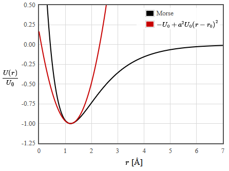
This potential looks like a parabola near the minimum, $U(r) \approx - U_0+ U_0a^2(r-r_0)^2+\cdots$, so a reasonable guess for a complete set of eigenfunctions that would describe the solutions to the Morse potential would be the harmonic oscillator eigenfunctions where the effective spring constant would be $2U_0a^2$. We seek a solution to the Schrödinger equation for the Morse potential of the form,
\begin{equation} \psi= c_0\phi_0+c_1\phi_1+c_2\phi_2+\cdots, \end{equation}where $\phi_i$ are the harmonic oscillator eigenfunctions and $c_i$ are unknown coefficients. Substitute this wave function into the time independent Schrödinger equation,
\begin{equation} H\psi= E\psi. \end{equation}Multiply the Schrödinger equation from the left by each of the harmonic oscillator wave functions and integrate over all space. This results in a set of $N$ algebraic equations.
\[ \begin{equation} \begin{matrix} \langle \phi_0 | H |\psi\rangle =E\langle\phi_0|\psi \rangle \\ \langle \phi_1 | H |\psi\rangle =E\langle\phi_1|\psi \rangle\\ \vdots \\ \langle \phi_N | H |\psi\rangle =E\langle\phi_N|\psi \rangle \end{matrix} \end{equation} \]By substituting in the form for $\psi$ from above, these equations can be written in matrix form,
\[ \begin{equation} \left[ \begin{matrix} H_{11} & H_{12} & \cdots & H_{1N} \\ H_{21} & H_{22} & \cdots & H_{2N} \\ \vdots & \vdots & \ddots & \vdots \\ H_{N1} & H_{N2} & \cdots & H_{NN} \end{matrix} \right] \left[ \begin{matrix} c_1 \\ c_2 \\ \vdots \\ c_N \end{matrix} \right] = E\left[ \begin{matrix} S_{11} & S_{12} & \cdots & S_{1N} \\ S_{21} & S_{22} & \cdots & S_{2N} \\ \vdots & \vdots & \ddots & \vdots \\ S_{N1} & S_{N2} & \cdots & S_{NN} \end{matrix} \right] \left[ \begin{matrix} c_1 \\ c_2 \\ \vdots \\ c_N \end{matrix} \right]. \end{equation} \]Here the elements of the Hamiltonian matrix and the overlap matrix are,
\[ \begin{equation} H_{ij}= \langle\phi_{i}|H|\phi_{j}\rangle \hspace{1cm}\text{and}\hspace{1cm} S_{ij}= \langle\phi_{i}|\phi_{j}\rangle =\delta_{ij}. \end{equation} \]Since the harmonic oscillator solutions are orthonormal, the overlap matrix $\textbf{S}$ is the identity matrix and the equations that need to be solved reduce to an eigenvalue problem,
\[ \begin{equation} \left[ \begin{matrix} H_{11} & H_{12} & \cdots & H_{1N} \\ H_{21} & H_{22} & \cdots & H_{2N} \\ \vdots & \vdots & \ddots & \vdots \\ H_{N1} & H_{N2} & \cdots & H_{NN} \end{matrix} \right] \left[ \begin{matrix} c_1 \\ c_2 \\ \vdots \\ c_N \end{matrix} \right] = E \left[ \begin{matrix} c_1 \\ c_2 \\ \vdots \\ c_N \end{matrix} \right]. \end{equation} \]This $N\times N$ Hamiltonian matrix has $N$ eigenvalues and their corresponding $N$ eigenvectors. The eigenvalue with the lowest energy is the best approximate ground state energy that can be found for the Morse potential using this set of $N$ harmonic oscillator wave functions. The corresponding eigenvector contains the coefficients $c_i$ needed to construct the ground state wave function $\psi= c_0\phi_0+c_1\phi_1+c_2\phi_2+\cdots+c_N\phi_N$. The other eigenvalues and their eigenvectors describe the excited states of the Morse potential.
Another class of problems that can be solved like this are potentials where $V(x)=\infty$ for $x<-L/2$ and for $x>L/2$. The time-independent Schrödinger equation for this case is,
\[ \begin{equation} -\frac{\hbar^2}{2m}\frac{d^2\psi}{dx^2}+V(x)\psi =E\psi . \end{equation} \]For these potentials we expand the wavefunction in terms of $N$ square-well eigenfunctions,
\begin{equation} \psi= c_1\phi_1+c_2\phi_2+c_3\phi_3+\cdots+c_N\phi_N, \end{equation}where $c_i$ are unknown coefficients and $\phi_i$ are the normalized square-well eigenfunctions,
\[ \begin{equation} \phi_n = \sqrt{\frac{2}{L}}\sin\left(n\pi\left(\frac{x}{L}+\frac{1}{2}\right)\right) \hspace{1cm}n=1,2,3,\cdots. \end{equation} \]The square-well eigenfunctions solve the Schrödinger equation for a potential $V(x)=0$. Substitute this wave function into the time-independent Schrödinger equation,
\begin{equation} H\psi= E\psi. \end{equation}Multiply the Schrödinger equation from the left by each of the square-well eigenfunctions and integrate from $-L/2$ to $L/2$. This results in a set of $N$ algebraic equations,
\[ \begin{equation} \begin{matrix} \langle \phi_1 | H |\psi\rangle =E\langle\phi_1|\psi \rangle \\ \langle \phi_2 | H |\psi\rangle =E\langle\phi_2|\psi \rangle\\ \vdots \\ \langle \phi_N | H |\psi\rangle =E\langle\phi_N|\psi \rangle \end{matrix} \end{equation} \].These equations can be written in matrix form,
\[ \begin{equation} \left[ \begin{matrix} H_{11} & H_{12} & \cdots & H_{1N} \\ H_{21} & H_{22} & \cdots & H_{2N} \\ \vdots & \vdots & \ddots & \vdots \\ H_{N1} & H_{N2} & \cdots & H_{NN} \end{matrix} \right] \left[ \begin{matrix} c_1 \\ c_2 \\ \vdots \\ c_N \end{matrix} \right] = E\left[ \begin{matrix} S_{11} & S_{12} & \cdots & S_{1N} \\ S_{21} & S_{22} & \cdots & S_{2N} \\ \vdots & \vdots & \ddots & \vdots \\ S_{N1} & S_{N2} & \cdots & S_{NN} \end{matrix} \right] \left[ \begin{matrix} c_1 \\ c_2 \\ \vdots \\ c_N \end{matrix} \right]. \end{equation} \]Here the elements of the Hamiltonian matrix and the overlap matrix are,
\[ \begin{equation} H_{mn}= \langle\phi_{m}|H|\phi_{n}\rangle \hspace{1cm}\text{and}\hspace{1cm} S_{mn}= \langle\phi_{m}|\phi_{n}\rangle. \end{equation} \]Since the square well eigenfunctions are orthonormal, the overlap matrix $\textbf{S}$ is the identity matrix. The matrix elements $H_{mn}$ are found by evaluating the following integral numerically.
\[ \begin{equation} H_{mn} = \int \limits_{-L/2}^{L/2}\frac{2}{L}\sin\left(m\pi\left(\frac{x}{L}+\frac{1}{2}\right)\right)\left(-\frac{\hbar^2}{2m}\frac{d^2}{dx^2}+V(x)\right)\sin\left(n\pi\left(\frac{x}{L}+\frac{1}{2}\right)\right)dx . \end{equation} \]The equations that need to be solved reduce to an eigenvalue problem,
\[ \begin{equation} \left[ \begin{matrix} H_{11} & H_{12} & \cdots & H_{1N} \\ H_{21} & H_{22} & \cdots & H_{2N} \\ \vdots & \vdots & \ddots & \vdots \\ H_{N1} & H_{N2} & \cdots & H_{NN} \end{matrix} \right] \left[ \begin{matrix} c_1 \\ c_2 \\ \vdots \\ c_N \end{matrix} \right] = E \left[ \begin{matrix} c_1 \\ c_2 \\ \vdots \\ c_N \end{matrix} \right]. \end{equation} \]This $N\times N$ Hamiltonian matrix has $N$ eigenvalues and their corresponding $N$ eigenvectors. The eigenvalue with the lowest energy is the best approximate ground state energy that can be found for the potential using this set of $N$ square well eigenfunctions. The corresponding eigenvector contains the coefficients $c_i$ needed to construct the ground state wave function $\psi= c_1\phi_1+c_2\phi_2+\cdots+c_N\phi_N$. The other eigenvalues and their eigenvectors describe the excited states of the potential.
The form below will construct the Hamiltonian matrix for a square well potential. The units of the matrix elements are eV.
|
The Hamiltonian matrix is,
1.13 Consider an electron moving in potential where $V(x)=\infty$ for $x<-L/2$ and for $x>L/2$. In the range $-L/2 < x < L/2$, the potential is $V(x)=5\exp\left(-\frac{10x^2}{L^2}\right)$ eV.
(a)Explain how the elements of the Hamiltonian matrix can be calculated. Calculate one element without using the app above.
(b) What are the first three eigenfunctions and their eigenenergies for this potential where $L=3$ nm?
1.14 (Old exam question) The starting point for the quantum description of an atom with $Z$ protons and $Z$ electrons is the many-electron Hamiltonian,
\begin{equation} H_{\text{me}}= - \sum \limits_{i=1}^Z \frac{\hbar^2}{2m_e}\nabla_i^2 - \sum \limits_{i=1}^Z \frac{Ze^2}{4\pi\epsilon_0 | \vec{r}_i |} + \sum \limits_{i\lt j}\frac{e^2}{4\pi\epsilon_0 |\vec{r}_i - \vec{r}_j | }. \end{equation}An approximate solution of the many-electron Hamiltonian for an atom can be found by neglecting the electron-electron interactions. The resulting Hamiltonian is called the reduced Hamiltonian. The reduced Hamiltonian is the sum of $Z$ identical atomic orbital Hamiltonians.
\begin{equation} H_{\text{red}}= \sum \limits_{i=1}^Z H_{\text{ao}}. \end{equation}(a) What is the atomic orbital Hamiltonian $H_{\text{ao}}$ for silicon $Z =$ 14?
$H_{\text{ao}}^{\text{Si}}=$
(b) The antisymmetrized solutions to the reduced Hamiltonian can be written as a Slater determinant. What is the Slater determinant for He $1s^2$?
$\Psi(\vec{r}_1,\vec{r}_1)=$