Sommerfeld expansion

The contribution of the electrons to any of the thermodynamic properties of a material can be calculated from the electron density of states. The density of states for a material can be determined by a band-structure calculation. It is possible to calculate a band structure yourself using a program like Quantum Espresso or many densities of states can be found at The Materials Project. Some example electron densities of states are listed below.

Al fcc, Au fcc, Cu fcc, Cr bcc, Li bcc, Na bcc, Pt fcc, W bcc, Si diamond, Fe bcc, Ni fcc, Co fcc, Mn bcc, Cr bcc, Gd hcp, Pd fcc, Pd₃Cr, Pd₃Mn, PdCr, PdMn, GaN, 6H SiC, GaAs, GaP, Ge, InAs, V bcc

A constant can be added to the energy and it is customary to set the Fermi energy to zero, $E_F = 0$. We will see that this choice has no effect on the outcome of the calculation.

When calculating the thermodynamic properties it is necessary to perform integrals for the electron density $n$ and the internal energy density $u$,

$$n =\int\limits_{-\infty}^{\infty}D(E)f(E)dE , \qquad u =\int\limits_{-\infty}^{\infty}ED(E)f(E)dE.$$ Arnold Sommerfeld recognized that there is a way to perform integrals of this form,

\[ \begin{equation} \int \limits_{-\infty}^{\infty} H(E)f(E)~dE, \end{equation} \]

where $f(E)$ is the Fermi function,

$$f(E) = \frac{1}{ \exp\left(\frac{E-\mu}{k_B T}\right)+1}.$$

and $H(E)$ is any function that goes to zero for large negative energies, $H(-\infty)=0$. The density of states $D(E)$ always goes to zero for large negative energies because there is always a finite lowest energy to a quantum system. The integrals for the electron density and internal energy density have the form that Sommerfeld considered.

Sommerfeld integrated once by parts,

\[ \begin{equation} \int \limits_{-\infty}^{\infty} H(E)f(E)~dE=K(\infty)f(\infty)-K(-\infty)f(-\infty)-\int \limits_{-\infty}^{\infty} K(E)\frac{df}{dE}dE, \end{equation} \]

where $K(E)$ is,

\[ \begin{equation} K(E) = \int \limits_{-\infty}^{E} H(E')~dE'. \end{equation} \]

The boundary terms vanish because $K(-\infty) = 0$ and $f(\infty) = 0$. The integral can then be written as,

\[ \begin{equation} \int \limits_{-\infty}^{\infty} H(E)f(E)~dE=-\int \limits_{-\infty}^{\infty} K(E)\frac{df}{dE}dE, \end{equation} \]

This is convenient because the derivative of the Fermi function is only nonzero in a region a few $k_BT$ wide around the chemical potential $\mu$, \[ \begin{equation} -\frac{df(E)}{dE} = \frac{\exp\left(\frac{E-\mu}{k_B T}\right)}{k_B T \left( \exp\left(\frac{E-\mu}{k_B T}\right)+1 \right)^2}. \end{equation} \]

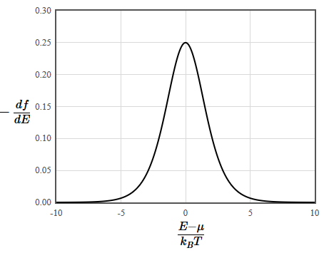
This means that only the states within a few $k_BT$ of the chemical potential are important for determining the thermodynamic properties of a material. The original integral can then be approximated by an integral over a small energy range and this can be evaluated numerically.

\[ \begin{equation} \int \limits_{-\infty}^{\infty} H(E)f(E)~dE \approx -\int \limits_{-10\mu/k_BT}^{10\mu/k_BT} K(E)\frac{df}{dE}dE. \end{equation} \]

This relationship was used to write programs to numerically calculate the temperature dependence of the electronic contribution to the thermodynamic properties of metals such as the chemical potential, the internal energy, the Helmholtz free energy density, the Grand potential density and the specific heat.

There were no computers when Sommerfeld was working on this problem so he expressed $K(E)$ as a Taylor expansion,

\[ \begin{equation} K(E) = K(\mu)+\frac{dK}{dE}\biggr\rvert_{E=\mu}(E-\mu)+\frac{1}{2}\frac{d^2K}{dE^2}\biggr\rvert_{E=\mu}(E-\mu)^2+\cdots = K(\mu)+H(\mu)(E-\mu)+\frac{1}{2}\frac{dH}{dE}\biggr\rvert_{E=\mu}(E-\mu)^2+\cdots. \end{equation} \]

Let $x = \frac{E-\mu}{k_BT}$, then the derivative of the Fermi function and the Taylor expansion can be written,

$$-\frac{df(x)}{dx} = \frac{e^x}{(1+e^x)^2},$$ $$K(x) = K(\mu)+k_BTH(\mu)x+k_B^2T^2\frac{1}{2}\frac{dH}{dE}\biggr\rvert_{E=\mu}x^2+\cdots,$$

and then he integrated term by term. Using the definite integrals,

\[ \begin{equation} \int \limits_{-\infty}^{\infty} \frac{e^x}{(1+e^x)^2}dx=1 \hspace{1.5cm} \int \limits_{-\infty}^{\infty} \frac{xe^x}{(1+e^x)^2}dx=0 \end{equation} \] \[ \begin{equation} \int \limits_{-\infty}^{\infty} \frac{x^2e^x}{(1+e^x)^2}dx=\frac{\pi^2}{3} \hspace{1.5cm} \int \limits_{-\infty}^{\infty} \frac{x^3e^x}{(1+e^x)^2}dx=0 \end{equation} \] \[ \begin{equation} \int \limits_{-\infty}^{\infty} \frac{x^4e^x}{(1+e^x)^2}dx=\frac{7\pi^4}{15} \hspace{1.5cm} \int \limits_{-\infty}^{\infty} \frac{x^5e^x}{(1+e^x)^2}dx=0 \end{equation} \]

The Sommerfeld expansion is,

\[ \begin{equation} \int \limits_{-\infty}^{\infty} H(E)f(E)~dE = K(\mu)+\frac{\pi^2}{6}(k_BT)^2\frac{dH}{dE}\biggr\rvert_{E=\mu}+\frac{7\pi^4}{360}(k_BT)^4\frac{d^3H}{dE^3}\biggr\rvert_{E=\mu}+\cdots. \end{equation} \]

The first two terms of the Sommerfeld expansion can be used to approximate the temperature dependence the thermodynamic properties of a material. These terms contain the density of states at the Fermi energy $D(E_F)$ and the derivative of the electron density of states at the Fermi energy $\frac{dD(E)}{dE}\Big{|}_{E=E_F}=D'(E_F)$. The parameters $D(E_F)$ and $D'(E_F)$ are enough to describe the electron density of states near the chemical potential. The formulas are the same for 1D, 2D and 3D.

Chemical potential μ Implicitly defined by \[ \begin{equation} n =\int \limits_{-\infty}^{\infty} D(E)f(E)dE \end{equation} \]	\[ \begin{equation} \mu \approx E_F-\frac{\pi^2}{6}(k_BT)^2\frac{D'(E_F)}{D(E_F)}\,[\text{J}] \end{equation} \]
Internal energy \[ \begin{equation} u= \int \limits_{-\infty}^{\infty} ED(E)f(E)~dE \end{equation} \]	\[ \begin{equation} u\approx\int\limits_{-\infty}^{E_F}ED(E)dE+\frac{\pi^2D(E_F)}{6}(k_BT)^2\,[\text{J m}^{-3}] \end{equation} \]
Specific heat \[ \begin{equation} c_v=\left(\frac{du}{dT}\right)_{V=\text{const}} \end{equation} \]	\[ \begin{equation} c_v\approx\frac{\pi^2D(E_F)}{3}k_B^2T\,\,[\text{J m}^{-3}\text{ K}^{-1}] \end{equation} \]
Entropy \[ \begin{equation} s=\int\frac{c_v}{T}dT \end{equation} \]	\[ \begin{equation} s\approx\frac{\pi^2D(E_F)}{3}k_B^2T\,\,[\text{J m}^{-3}\text{ K}^{-1}] \end{equation} \]
Helmholtz free energy \[ \begin{equation} f=u-Ts \end{equation} \]	\[ \begin{equation} f\approx\int\limits_{-\infty}^{E_F}ED(E)dE-\frac{\pi^2D(E_F)}{6}(k_BT)^2\,[\text{J m}^{-3}] \end{equation} \]

The density of states at the Fermi energy and the derivative of the density of states at the Fermi energy are given for a few materials in the table below.

	$D(E_F)$ J^-1 m^-3	$D'(E_F)$ J^-2 m^-3
Al	1.3 × 10⁴⁷	-5.8 × 10⁶⁵
Cu	3.24 × 10⁴⁷	-1.2 × 10⁶⁵
Cr	5.2 × 10⁴⁷	9.4 × 10⁶⁵
Li	1.5 × 10⁴⁷	7.0 × 10⁶⁵
Na	8.4 × 10⁴⁶	2.2 × 10⁶⁵
V	9.9 × 10⁴⁷	-8.9 × 10⁶⁵

It seems like we need to know $E_F$ and $u_0 =\int\limits_{-\infty}^{E_F}ED(E)dE$ in order to proceed but there is a subtle issue with these quantities. The core electrons are rarely included in a band structure so that $D(E)$ just includes the states around the Fermi energy. A different calculation might describe the states around the Fermi energy the same but include more bands so that the energy difference from the lowest occupied state to the highest occupied state (the Fermi energy) is different for the two calculations. For this reason, sometimes the cohesive energy is introduced to provide a reference energy. The cohesive energy is the energy that is needed to take a crystal apart by expanding the lattice constant. The atoms stay in the same arrangement, just the distances between them are increased until there is negilible interaction between the atoms. The atoms could be rearranged into a different crystal structure while they are far apart from each other and then allowed to move together to the equilibrium distance for the new crystal structure. You can then use the cohesive energy of each crystal structure for $u_0$ and set $E_F =0$.

The mathematical functions that can be used are list below. Multiplication must be specified with a '*' symbol, 3*cos(x) not 3cos(x). Powers are specified with the 'pow' function: x³ is pow(x,3) or x**3 not x^3.
<table align='center'><tr><td><ul><li>abs(x) - absolute value</li><li>acos(x) - inverse cosine</li><li>acosh(x) - inverse hyperbolic cosine</li>
<li>asin(x) - inverse sine</li><li>asinh(x) - inverse hyperbolic sine</li><li>atan(x) - inverse tangent</li><li>atanh(x) - inverse hyperbolic tangent</li><li>cos(x) - cosine</li><li>cosh(x) - hyperbolic cosine</li>
<li>exp(x) - et</li></ul></td>
<td><ul><li>log(x) - natural logarithm</li><li>pi = 3.141592653589793</li><li>pow(t,y) - compute ty</li><li>round(x) - round to the nearest integer</li>
<li>sin(x) - sine</li><li>sinh(x) - hyperbolic sine</li><li>sqrt(x) - square root</li><li>tan(x) - tangent</li><li>tanh(x) - hyperbolic tangent</li><li>H(x) - Heaviside function = 0 for x < 0, 1 for x > 0</li></ul></td></tr></table>
 
<a href="https://lampz.tugraz.at/~hadley/physikm/script/intro/vectorscript.en.php?print">Vector functions</a> 
<table align='center'><tr><td><ul><li>cross(A,B) - cross product</li><li>dot(A,B) - scalar product of two vectors </li><li>dot(a,B) - scalar a times vector B</li><li>length(A) - length of a vector</li></ul></td><td valign="top"><ul><li>unit(A) - unit vector in direction of A</li><li>vadd(A,B) - vector addition A + B</li><li>vsub(A,B) - vector subtraction A -B</li></ul></td></tr></table>

● print(x) - Text or variables can be printed to the Script Output box with the print(x) function. Text should be put in quotes, print("Print some text"). The value of variable x can be printed with print(x) and text can be mixed with variables by concatenating them together with a + sign, print("The length is "+x+" m.").

kB = 1.380649E-23; // [J/K] Boltzmann's constant e = 1.602176634E-19; // [C] elementary charge pi = 3.141592653589793; D_EF = 1.3E47; // density of states at EF [J^(-1) m^(-3)] dDdE_EF = -5.8E65; // erivative of the density of states at EF [J^(-2) m^(-3)] T = 300; // temperature [K] EF = 0; // you can choose the value of EF u0 = 0; // u(T=0) mu = EF - (pipi/6)pow(kBT,2)(dDdE_EF/D_EF); //chemical potential [J] mu_eV = mu/e; //chemical potential [eV] u = u0 + (pipi/6)pow(kBT,2)D_EF; // internal energy density J/m^3 cv = (pipi/3)(kBkBT)D_EF; // specific heat J/(K m^3) s = (pipi/3)(kBkBT)D_EF; ; // entropy density J/(K m^3) f = u0 - (pipi/6)pow(kBT,2)D_EF; // Helmholtz free energy density J/m^3
Script Output

Sommerfeld-Entwicklung: Appendix C in Festkörperphysik, R. Gross und A. Marx (Available to TU Graz students through the TU Graz library).
A good source for the density of states of different materials is Springer Materials.
Plots of the band structure and the density of states for most metals can be found in: D. A. Papaconstantopoulos, Handbook of the band structure of elemental solids, Plenum Press (1986).
Sommerfeld Expansion, Wikipedia