![]()
PHY.K02UF Molecular and Solid State Physics
|
| |||
PHY.K02UF Molecular and Solid State Physics | ||||
Often in solid state physics we need to work with periodic functions. For instance, the electron density in a crystal is a three-dimensional periodic function. Periodic functions can be described using a Fourier series. Fourier series in one dimension will be discussed first and then the concept will be generalized to two and three dimensions.
Fourier series in one dimension
For a one-dimensional function $f(x)$ with periodicity $a$, a Fourier series is often written in terms of sines and cosines,
$$f(x)= c_0 +\sum\limits_{n=1}^{\infty}\left(c_n\cos(2\pi nx/a) + s_n\sin(2\pi nx/a)\right).$$Here $c_n$ and $s_n$ are constants. The periodic function is a constant $c_0$ plus sinusiodal functions with wavelengths $a/n$. The terms with $n=1$ is call the fundamental component and the terms with $n > 1$ are the harmonics. If the function $f(x)$ is known, the constants can be calculated with the formulas,
$$c_n = \frac{2}{a}\int\limits_{0}^af(x)\cos(2\pi nx/a)dx,$$ $$s_n = \frac{2}{a}\int\limits_{0}^af(x)\sin(2\pi nx/a)dx.$$These formulas can be seen as the projection of $f(x)$ onto $\cos(2\pi nx/a)$ and $\sin(2\pi nx/a)$. If $f(x)$ is a square wave function,
| $\frac{f(x)}{f_0}$ | |
$x$ |
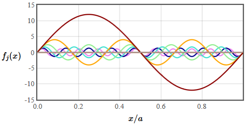
the coefficients are $c_n = \frac{2}{\pi n}\sin\left(\frac{\pi n}{2}\right)$, $s_n=0$. The form below will show you the waveform when the Fourier series is truncated at $n_{\text{max}}$.
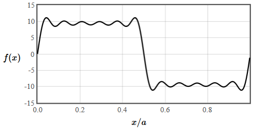
The resulting function $f(x)$ depends on the amplitudes of the harmonics as well as the phase between the harmonics. The figure below shows the amplitude and the phase of the harmonics that make up a square wave.
Sometimes a Fourier series is written in terms of the amplitudes and phases as,
$$f(x) = A_0 +\sum\limits_n A_n\left(\cos(\theta_n)\cos (2\pi nx/a)+\sin(\theta_n)\sin (2\pi nx/a)\right),$$where $c_n=A_n\cos(\theta_n)$ and $s_n=A_n\sin(\theta_n)$. Follow this link for more examples of Fourier series.
To make the generalization of a Fourier series to two and three dimensions, it is convenient to express the sine and cosine terms as complex exponentials, $\sin(x) = (e^{ix}-e^{-ix})/(2i)$, $\cos(x) = (e^{ix}+e^{-ix})/2$ and to define $G_n=2\pi n/a$. The Fourier series can then be written compactly as,
$$f(x) = \sum\limits_{n=-\infty}^{\infty}f_{G_n}e^{iG_nx},\qquad f_{G_n} = \frac{c_n}{2} - i\frac{s_n}{2}.$$At first this seems more complicated because we have replaced friendly functions like $\sin(x)$ and $\cos(x)$ with a sum of complex exponentials with complex coefficients. However, this is a mathematically convenient form because exponential functions are easy to integrate and to differentiate. They can also be easily multiplied together by adding the exponents. To plot the series we can convert back to sines and cosines using Euler's formula, $e^{ix}= \cos(x)+i\sin(x)$.
The form below lets you compose a real periodic function from the Fourier components. The period of the function is $a=1$.
| $f(x)$ | |
$x$ |
The real part of the Fourier coefficients encodes the cosine components and the imaginary part of the Fourier coefficients encodes the sine components.
The generalization of a Fourier series to an arbitrary number of dimensions is,
$$f(\vec{r})=\sum \limits_{\vec{G}} f_{\vec{G}}\exp \left(i\vec{G}\cdot\vec{r}\right),$$where the sum is over the reciprocal lattice vectors $\vec{G}$ of the Bravais and $f_{\vec{G}}$ are complex coefficients (sometimes called the structure factors). If $f(\vec{r})$ is a real function, then $f_{-\vec{G}}=f_{\vec{G}}^*$.
We will next define the reciprocal latice vectors $\vec{G}$ that are needed for a Fourier series.