![]()
PHY.K02UF Molecular and Solid State Physics
|
| |||
PHY.K02UF Molecular and Solid State Physics | ||||
Often in solid state physics we need to work with functions that are periodic. For instance, the electron density in a crystal is a three-dimensional periodic function. Periodic functions can be described using a Fourier series. For a one-dimensional function $f(x)$ with periodicity $a$, a Fourier series is often written in terms of sines and cosines,
$$f(x)= c_0 +\sum\limits_{n=1}^{\infty}\left(c_n\cos(2\pi x/a) + s_n\sin(2\pi x/a)\right).$$Here $c_n$ and $s_n$ are constants. The periodic function is a constant $c_0$ plus sinusiodal functions with wavelengths $a/n$. The terms with $n=1$ is call the fundamental component and the terms with $n > 1$ are the harmonics. If the function $f(x)$ is known, the constants can be calculated with the formulas,
$$c_n = \frac{2}{a}\int\limits_{0}^af(x)\cos(2\pi nx/a)dx,$$ $$s_n = \frac{2}{a}\int\limits_{0}^af(x)\sin(2\pi nx/a)dx.$$If $f(x)$ is a square wave function,
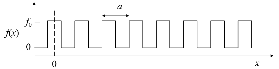
the coefficients are $c_n = \frac{2}{\pi n}\sin\left(\frac{\pi n}{2}\right)$, $s_n=0$. The form below will show you the waveform when the Fourier series is truncated at $n_{\text{max}}$.
To make the generalization of a Fourier series to two and three dimensions, it is convenient to express the sine and cosine terms as complex exponentials, $\sin(x) = (e^{ix}-e^{-ix})/(2i)$, $\cos(x) = (e^{ix}+e^{-ix})/2$ and to define $G_n=2\pi n/a$. The Fourier series can then be written compactly as,
$$f(x) = \sum\limits_{n=-\infty}^{\infty}f_{G_n}e^{iG_nx},\qquad f_{G_n} = \frac{c_n}{2} + i\frac{s_n}{2}.$$At first this seems more complicated because we have replaced friendly functions like $\sin(x)$ and $\cos(x)$ with a sum of complex exponentials with complex coefficients. However, this is a mathematically convenient form because exponential functions are easy to integrate and to differentiate. They can also be easily multiplied together by adding the exponents. To plot the series we can convert back to sines and cosines using Euler's formula, $e^{ix}= \cos(x)+i\sin(x)$.
The generalization of a Fourier series to an arbitrary number of dimensions is,
$$f(\vec{r})=\sum \limits_{\vec{G}} f_{\vec{G}}\exp \left(i\vec{G}\cdot\vec{r}\right),$$where the sum is over the reciprocal lattice vectors $\vec{G}$ of the Bravais and $f_{\vec{G}}$ are complex coefficients (called the structure factors). If $f(\vec{r})$ is a real function, then $f_{-\vec{G}}=f_{\vec{G}}^*$.
Every periodic function can be associated with a Bravais lattice. There is 1 Bravais lattice in one dimension, there are 5 Bravais lattices in two dimensions and there are 14 Bravais lattices in three diemensitons. You can think of any periodic function as being defined in by a primitive unit cell that is repeated at every point of the Bravais lattice.
Using the definition of a reciprocal lattice vector,
$$\vec{G}=\nu_1\vec{b}_1+\nu_2\vec{b}_2+\nu_3\vec{b}_3\hspace{1.5 cm}\nu_1,\nu_2,\nu_3 = \cdots ,-2,-1,0,1,2,\cdots$$the Fourier series can be rewritten in terms of the primitive reciprocal lattice vectors, $\vec{b}_j$.

An example of a real periodic function that has an orthorhombic Bravais lattice can be constructed using the reciprocal lattice vectors 100, -100, 010, 0-10, 001, 00-1. If for all of these reciprocal lattice points $f_{\vec{G}}=1$, then the periodic function is,

In a similar manner, periodic functions with a bcc, fcc, or hexagonal Bravais lattice can be constructed.
| bcc: |  |
| fcc: |  |
| hexagonal: |  |
If the periodic function f(r) is known, the Fourier coefficients fG can be determined by multiplying both sides of a Fourier series by exp(-iG'·r) and integrating over a primitive unit cell.

The left-hand side is the Fouier transform of the function f(r) restricted to a unit cell. On the right-hand side, only the term where G = G' contributes and the integral evaluates to fG times the volume V of the primitive unit cell.
The function fcell(r) = f(r) within the primitive unit cell and is zero outside the primitive unit cell. The Fourier coefficient fG is the Fourier transform of the function fcell(r) divided by the volume.
Example 1: cubes repeated on a bcc lattice
Cubes are arranged on a bcc lattice such that the corners of the cubes just touch.
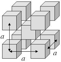
A three-dimensional periodic function f is defined such that it has a constant value C inside the cubes and is zero outside the cubes. This function can be expressed as a Fourier series,
The Fourier coefficients fG are given by,
The cube at the origin lies entirely within the Wigner-Seitz cell and the function f is zero outside the cube so we just need to integrate over the cube. The integrals over x, y and z are easily performed.
This result can readily be generalized to any rectangular cuboid with dimensions Lx×Ly×Lz that is repeated on any three-dimensional Bravais lattice. As long as a primitive unit cell can be defined such that the cuboid is entirely within the cell, the Fourier series for a function that has the value C inside the cuboids and zero outside the cuboids is,
Here V is the volume of the primitive unit cell.
Example 2: spheres on an fcc lattice
Spheres of radius R are arranged on a fcc lattice.
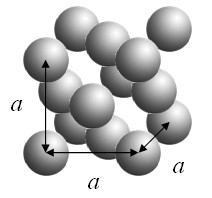
A three-dimensional periodic function f is defined such that it has a constant value C inside the spheres and is zero outside the spheres. This function can be expressed as a Fourier series,
The Fourier coefficients fG are given by,
As long as the spheres do not overlap, a primitive unit cell can be defined so that the sphere at the origin lies entirely within the primitive unit cell. Since the function f is zero outside sphere, we just need to integrate over the sphere.
The integral over φ is easily performed.
Recognizing that,
the integral over θ can be performed.
Finally, performing the integral over r,
As long as the spheres do not overlap, the Fourier series for spheres repeated on any Bravais lattice is,
Example 3: Total electron density
The total electron density in a crystal is a periodic function. Most of the electrons in a solid are core electrons that are very tightly bound to the nuclei. To a good approximation, the total electron density of an atom can be described by a Gaussian function $\frac{Z}{r_0^3 \pi^{3/2}}\exp (-r^2/r_0^2)$, where $Z$ is the number of electrons of the atom. The integral of this function over all space is $Z$. Typically the width $r_0$ of the Gaussian is so much smaller than the lattice constant $a$ the that the integral of this function over a unit cell is also about $Z$. The electron density of the basis of a crystal is,
\[ \begin{equation} n_{u.c.}(\vec{r})=\sum \limits_j \frac{Z_j}{r_{0j}^3 \pi^{3/2}}\exp \left(-\frac{(\vec{r}-\vec{r}_j)^2}{r_{0j}^2}\right), \end{equation} \]where $j$ sums over the atoms in the basis and $\vec{r}_j$ is the position of atom $j$.
The structure factor can be found by multiplying both sides of this equation by $\exp (-i\vec{G}\cdot\vec{r})$ and integrating over a unit cell.
\[ \begin{equation} n_{\vec{G}}=\frac{1}{V_{u.c.}}\sum \limits_j Z_j\exp \left(-\frac{r_{0j}^2G^2}{4}\right)\exp (-i\vec{G}\cdot\vec{r}_j). \end{equation} \]The square of the structure factor $|n_{\vec{G}}|^2$ is proportional to the intensity of a diffraction peak in an x-ray diffraction experiment. Since the volume of the unit cell is the same for all of the structure factors and only their ratio is important for x-ray diffraction, it is usual to leave the factor of the volume of the unit cell out and give the structure factor as,
\[ \begin{equation} n_{\vec{G}}=\sum \limits_j Z_j\exp \left(-\frac{r_{0j}^2G^2}{4}\right)\exp (-i\vec{G}\cdot\vec{r}_j). \end{equation} \]The structure factor for $\vec{G}=0$ is the number of electrons per unit cell,
\[ \begin{equation} n_{\vec{G}=0}=\sum \limits_j Z_j. \end{equation} \]Since the Gaussians are sharply peaked around the nuclei, sometimes the electron density is approximated by collection of $\delta$-functions,
\[ \begin{equation} n_{u.c.}(\vec{r})=\sum \limits_j Z_j\delta(\vec{r}-\vec{r}_j). \end{equation} \]In this case, the structure factors are,
\[ \begin{equation} n_{\vec{G}}=\sum \limits_j Z_j\exp (-i\vec{G}\cdot\vec{r}_j). \end{equation} \]
Example 4: The molecular orbital Hamiltonian
An important periodic function is the periodic potential that appears in the molecular orbital Hamiltonian for a crystal. For a crystal containing only one atom in the basis, the potential is,
\[ \begin{equation} U(\vec{r})=-\frac{Ze^2}{4\pi \epsilon_0}\sum \limits_j\frac{1}{|\vec{r}-\vec{r}_j|}. \end{equation} \]Here $\vec{r}_j$ are the positions of the atoms. The periodic potential is formed by the Coulomb potentials of the nuclei each with a positive charge of $Ze$. The Fourier series for this potential is,
\[ \begin{equation} U(\vec{r})=-\frac{Ze^2}{V_{u.c.} \epsilon_0}\sum \limits_{\vec{G}}\frac{\exp (i\vec{G}\cdot\vec{r})}{|\vec{G}|^2}. \end{equation} \]
Example 5: Muffin tin potentials
A muffin tin is used to bake muffins.

In solid state physics, a 2-d muffin tin potential is a potential consisting of a lattice of circular regions. Within the circular regions the potential is a Coulomb potential with the form -Ze²/(4πεr) and between the circular regions the potential is constant. The constant is chosen so that there is no discontinuity in the potential. This potential looks like a muffin tin.
In three dimensions, a muffin tin potential U(r) is a lattice of spherical regions where the potential inside the the spheres is -Ze²/(4πεr) and outside the spheres the potential is constant.
The integral that must be performed to determine the Fourier coefficients is,
The first term is the radial Fourier transform of the Coulomb potential and the second term adds a constant value to the potential in the spherical regions to match the Coulomb potential to the zero potential outside the spherical regions.
The Fourier series for a muffin tin potential is,
$$U(\vec{r})=\frac{Ze^2}{V\epsilon_0} \sum\limits_{\vec{G}}\left(\frac{\cos(|G|R)-1}{|G|^2}+\frac{\sin(|G|R)-|G|R\cos(|G|R)}{R|G|^3}\right)\exp\left(i\vec{G}\cdot\vec{r}\right).$$
Example 6: circles on a 2-d Bravais lattice
Consider a periodic function defined by non-overapping circles arranged on a 2-D Bravais lattice.

A function f is defined such that it has a constant value C inside the circles and is zero outside the circles. As long as the circles do not overlap, a primitive unit cell can be defined so that the circle at the origin lies entirely within the primitive unit cell. Since the function f is zero outside circle, we just need to integrate over the circle. The Fourier coefficients fG are given by,
Here A is the area of the primitive unit cell and R is the radius of the circles. Performing the integral over θ.
Here J0 is the zeroth order Bessel function. Integrating over r yields,
Here J1 is the first order Bessel function. As long as the circles do not overlap, the Fourier series for circles repeated on any 2-D Bravais lattice is,
Example 7: parallelograms repeated on a 2-D Bravais lattice
Consider a periodic function defined by non-overapping parallelograms arranged on a 2-D Bravais lattice.

A function f is defined such that it has a constant value C inside the parallelograms and is zero outside the parallelograms. As long as the parallelograms do not overlap, a primitive unit cell can be defined so that the parallelogram at the origin lies entirely within the primitive unit cell. Since the function f is zero outside parallelogram, we just need to integrate over the parallelogram. The Fourier coefficients fG are given by,
Here A is the area of the primitive unit cell. b and h are shown in the drawing. Performing the integral over y,

Integrating over x yields,
As long as the parallelograms do not overlap, the Fourier series for parallelograms repeated on any 2-D Bravais lattice is,

This includes the results for squares and rectangles as special cases (tan(0) = 0). e.g. rectangle: