Complex exponential functions will be used to describe the atomic motion. The relationship between sinusoidal motion and circular motion in the complex plane is given by Euler's formula.

Your browser does not support the canvas element.

\[ \begin{equation} \large \qquad e^{i\omega t} = \cos\omega t + i \sin\omega t \end{equation} \]

The red ball represents the position of the complex number $e^{i\omega t}$ as it moves through the complex plane with real numbers plotted horizontally and imaginary number plotted vertically. The black circle is the unit circle. The blue ball represents the position of $\cos \omega t$ and the green ball represents the position of $i\sin \omega t$. The simulation on the left is a graphical representation of the formula on the right.

Oscillations that can be described by $\sin \omega t$ or $\cos \omega t$ are called harmonic oscillations. From the simulation it is clear that there is a relationship between circular motion and harmonic oscillations. If you look at the motion of the red ball looking down at the complex plane, it moves in a circle but if you look at the motion of the red ball from the side (viewing in the direction of the imaginary axis), it executes harmonic motion.

The relationship between circular motion and harmonic oscillations is described easily using complex numbers. Sometimes when we observe a harmonic oscillation it is convenient to imagine that we are looking at circular motion from the side. We can't measure the component of the motion in the imaginary direction; we just imagine it.

Oscillations of a mass on a linear spring

Consider a mass $m$ connected to a linear spring with a spring constant $C$. (We will use $C$ for spring constant in this section since $k$ is reserved for wavenumbers.) The differential equation that describes the motion is,

$$m\frac{d^2y}{dt^2}=- Cy.$$

The solution to this differential equation can be written either in terms of $y(t)=A\sin(\omega t+ \delta)$ or $y(t)=A\cos(\omega t+ \delta)$ where $A$ is the amplitude of the oscillations, $\omega$ is the angular frequency, $t$ is the time and $\delta$ is a phase factor that would be set by the initial conditions.

It is also possible to imagine that the imaginary axis points into the screen and the mass is executing circular motion in the complex plane of the form, $Ae^{i\omega t}$. Substitute this form into the differential equation,

$$-\omega^2 mAe^{i\omega t}=- CAe^{i\omega t}.$$

This demonstrates that the complex form is a solution to the differential equation with the expected angular frequency,

$$\omega = \sqrt{\frac{C}{m}}.$$

In general, the amplitude $A$ can be a complex number. For instance, $y(t)= (1+i)e^{i\omega t}$ is a solution. The complex number can be written in polar form $(1+i)=\sqrt{2}e^{i\pi /4}$ and exponentials can be combined, $y(t) = \sqrt{2}e^{i(\omega t +\frac{\pi}{4})}$. The motion along the real axis that would be observed in this case is $y(t) = \sqrt{2}\cos(\omega t +\frac{\pi}{4})$. Thus, a complex amplitude $A$ contains the ampltude and the phase of the solution.

Normal modes of a simple system

Consider two identical masses $M$ connected by two identical springs $C$ that are confined to move in one dimension.

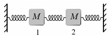
The differential equations that describe this motion are,

$$M\frac{d^2u_1}{dt^2} = -Cu_1 + C(u_2 - u_1),$$ $$M\frac{d^2u_2}{dt^2} = -Cu_2 + C(u_1 - u_2),$$

where $u_1$ and $u_2$ are the displacements of the masses from their equilibrium positions. In a normal mode, both masses will oscillate at the same frequency, $u_1= A_1e^{i\omega t}$ and $u_2= A_2e^{i\omega t}$. Substituting this form into the differential equations yields,

$$-\omega^2MA_1e^{i\omega t} = -CA_1e^{i\omega t} + C(A_2e^{i\omega t} - A_1e^{i\omega t}),$$ $$-\omega^2MA_2e^{i\omega t} = -CA_2e^{i\omega t} + C(A_1e^{i\omega t} - A_2e^{i\omega t}).$$

These equations can be written in matrix form,

\begin{equation} -\omega^2M\left[ \begin{matrix} A_1 \\ A_2 \end{matrix} \right]=\left[ \begin{matrix} -2C & C \\ C & -2C \end{matrix} \right]\left[ \begin{matrix} A_1 \\ A_2 \end{matrix} \right]=0. \end{equation}

The eigenvectors of a 2 × 2 matrix with the same values along the diagonal and the same values of the off-diagonal elements,

\begin{equation} \left[ \begin{matrix} a & b \\ b & a \end{matrix} \right] \end{equation}

are

\begin{equation} \left[ \begin{matrix} 1 \\ 1 \end{matrix} \right]\quad\text{with eigenvalue}\quad a+b \quad \text{and}\quad \left[ \begin{matrix} 1 \\ -1 \end{matrix} \right]\quad\text{with eigenvalue}\quad a-b. \end{equation}

The normal modes are an in-phase mode where the masses move together,

\begin{equation} \omega^2M\left[ \begin{matrix} 1 \\ 1 \end{matrix} \right]=C\left[ \begin{matrix} 1 \\ 1 \end{matrix} \right]\quad\rightarrow\quad \omega= \sqrt{\frac{C}{M}}, \end{equation}

and an out-of-phase mode where the masses move in opposite directions, \begin{equation} \omega^2M\left[ \begin{matrix} 1 \\ -1 \end{matrix} \right]=3C\left[ \begin{matrix} 1 \\ -1 \end{matrix} \right]\quad\rightarrow\quad \omega= \sqrt{\frac{3C}{M}}. \end{equation}